8  Timeline Analysis

Working Contents

library(jsonlite)
library(tidyverse)
library(DT)

repo <- "~/Workspaces/github/open-source-rover/build/results/"
file <- "query_scenario_move_v2.json"
filepath <- paste0(repo,file)
jsondata <- fromJSON(filepath)

colnum <- ncol(jsondata$results$bindings)
df <- data.frame(matrix(rep(NA, colnum), nrow=1))[numeric(0), ]
colnames(df) <- c(names(jsondata$results$bindings))

for (i in 1:nrow(jsondata$results$bindings)) {
  for (j in 1:colnum) {
    df[i,j] <- jsondata$results$bindings[i,j]$value
  }
}

# df <- df %>%
#   add_column(value = c(0,1,1,1,0))

# df$t <- as.numeric(df$t)
df$t <- as.numeric(df$time)
df$value <- as.numeric(df$value)

8.0.1 calcurate duration and endtime

# t_end[task_i] = t_start[task_i+1]

df_task <- df %>% 
  distinct(task, .keep_all = TRUE) %>%
  select(f2_id, f2_cname, task, t, f3_id)

df_task$t2 <- c(df_task$t[-1],df_task$t[nrow(df_task)]+2)

df$t2 <- df_task$t2[match(df$f2_id,df_task$f2_id)]

ypos <- max(df$value) + 1
dy <- 0.2
  
df2 <- data.frame(
   sv = df$statevariable,
   activity = paste0(df$f2_id,":",df$f2_cname),
   start_time=as.numeric(df$t),
   end_time=as.numeric(df$t2),
   state_value=as.numeric(df$value)
)

df2 %>% 
    ggplot(aes(start_time, state_value)) + 
    geom_point(aes(color = sv)) +
    geom_line(aes(color = sv)) +
    ggchicklet:::geom_rrect(
      aes(
        xmin = start_time,
        ymin = ypos,
        xmax = end_time,
        ymax = ypos+dy,
        fill = activity,
      ),
      r = unit(0.5, 'npc'),
      alpha = 0.5
    )+
   scale_x_continuous(
    breaks = seq(0, 10, 2),
    position = 'bottom'
    )

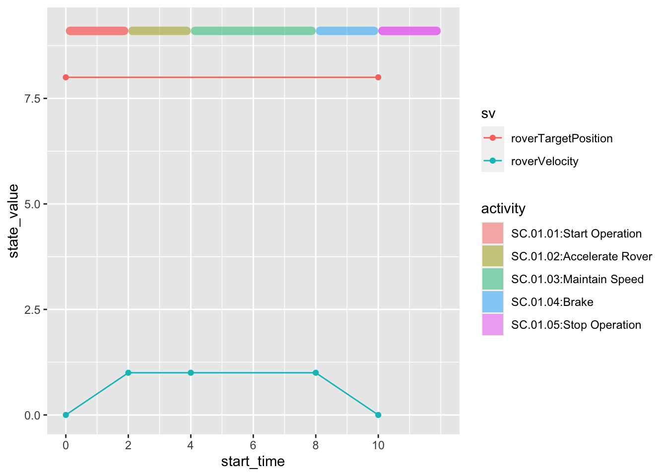
p<-df2 %>% 
    ggplot(aes(start_time, state_value)) + 
    geom_point(aes(color = sv)) +
    geom_line(aes(color = sv)) +
    geom_rect(
      aes(
        xmin = start_time,
        ymin = ypos,
        xmax = end_time,
        ymax = ypos+dy,
        fill = activity
      ),
      alpha = 0.5
    ) + 
    scale_x_continuous(
      breaks = seq(0, 10, 2),
      position = 'bottom'
      )

library(plotly)
ggplotly(p)

8.0.2 Using Gantt Chart

library(ganttrify)


df_project <- data.frame(
   wp = "scenario",
   activity = paste0(df_task$f2_id,":",df_task$f2_cname),
   start_date=as.numeric(df_task$t),
   end_date=as.numeric(df_task$t2)
)

colnum <- length(unique(df$wp))
colpal <- MetBrewer::met.brewer(name="VanGogh1", n=colnum)
colour_palette <- colpal

  
g <- ganttrify::ganttrify(
    project = df_project,
    # spots = ganttrify::test_spots_date_month,
    colour_palette = colpal,
    exact_date = FALSE,
    month_number_label = TRUE,
    month_date_label = FALSE,
    x_axis_position = "bottom",
    # project_start_date = startday,
#    font_family = font,
    size_wp = 6,
    hide_wp = TRUE,
#    by_date = TRUE,
#    mark_quarters = TRUE,
#    mark_years = TRUE,
#    month_breaks = 1,
    line_end = "round",
    axis_text_align = "left")

plot(g)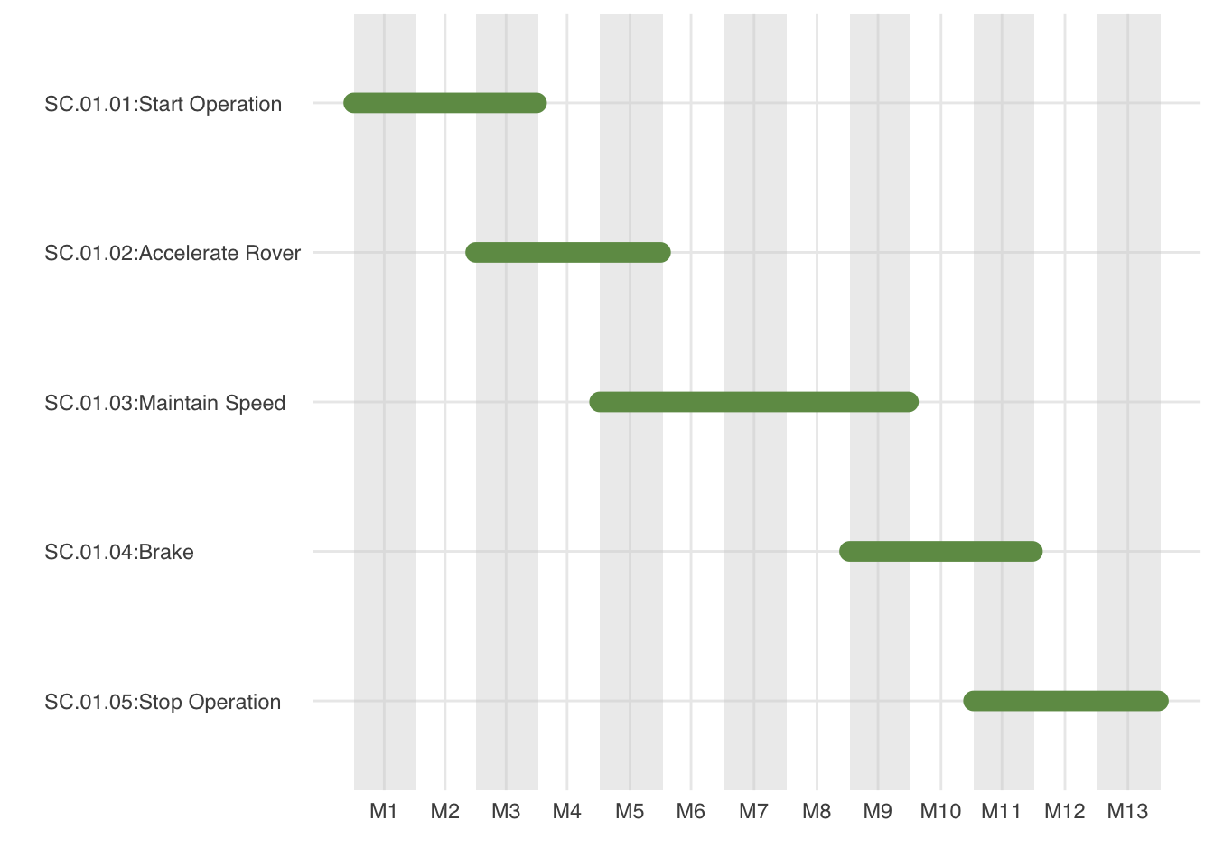

8.1 Generate Timeline file for modelica

df_timeline <- df %>% 
  filter(statevariable == "roverVelocity") %>%
  select(time, statevariable, value)
  
outputfile <- "~/Workspaces/openmodelica-docker-start/om-develop/timeline.txt"

txt <- "#1\n"
txt <- paste0(txt, "double Tab1(",nrow(df_timeline),",2)\n")
for( i in 1:nrow(df_timeline)){
  txt <- paste0(txt, df_timeline$time[i]," ",df_timeline$value[i],"\n")
}
cat(file = outputfile, txt)

8.2 Execute Modelica

## need some code